TUTORIAL - Measuring emission line fluxes with Python and deriving gas properties

Luke Holden - 30th January 2023

Emission lines are a key tool used in many areas of astrophysical research, and are one of the principal ways that we can investigate the properties and nature of the narrow line regions (NLRs) of active galaxies. Therefore, understanding how to derive line fluxes from spectra - and how these may be used to derive information about the line-emitting gas - is essential.

In this tutorial, I will show you how to fit emission lines in an SDSS active galaxy spectrum, and how the resulting line fluxes and ratios can be used to derive the electron density of the gas. It is important to note that the focus here is on giving a basic introduction to fitting lines and producing line fluxes - in reality, care must be taken when fitting emission lines (as they may require complex modelling with multiple components) and when measuring real electron densities (see Holden et al. 2023).

Throughout, I assume a prior familiarity with Python, as well as an undergraduate-level understanding of emission line and atomic physics.

Working with spectra and measuring line fluxes

In order to derive information about the physical conditions of gas, we first need to load in the spectrum, select emission lines and measure their line fluxes - that is the focus of this section.

Loading the SDSS spectral data and file headers

First, lets load in the Python modules that we'll be using:


                import numpy as np 

                import matplotlib.pyplot as plt 

                from astropy.io import fits 

                from astropy.modeling import models,fitting

Next, lets load in the .fits file of the galaxy we'll be looking at (SDSS-51959-0541-100), which can be found here.

SDSS spectrum files contain three different arrays for each object: the observed spectrum (in terms of the flux density: 10^-17 erg cm²s^-1Å^-1) the continuum-subtracted spectrum (the continuum is modelled by a polynomial), and the flux uncertainty associated with the spectrum. Here, we'll choose the first array (the observed spectrum):


                hdul = fits.open('spSpec-51959-0541-100.fit') 

                data = hdul[0].data 

                flux = data[0,:]

We also need to load in the .fits file header, which contains information about the object such as its redshift and world coordinate system (WCS). For spectra, the WCS is used to assign each data point a wavelength value - this is done using the CRVAL (starting wavelength) and CDELT (wavelength step per data point) parameters.


                # open .fits file header and create wavelength array (in angstroms) from WCS 

                hdr=fits.getheader('spSpec-51959-0541-100.fit')  

                crval=hdr['COEFF0'] 

                cdelt=hdr['COEFF1'] 

                pix = np.arange(0,len(data[0,:])) 

                w = 10**(hdr['COEFF0'] + hdr['COEFF1']*pix) 

                

                # get the redshift of the object from the .fit file header 

                z = hdr['Z'] 

                print("redshift = ", z) 

                >redshift =  0.0267809

Great - we now have the spectrum loaded in, and have arrays for the flux density and wavelength, as well as the object's redshift. Let's plot the spectrum and have a look:


                fig = plt.figure(figsize=(14,7)) 

                plt.step(w, flux, where='mid', color='k') 

                plt.xlabel(r"Wavelength ($\AA$)", fontsize=18) 

                plt.ylabel(r"Flux (erg cm$^{-2}$ s$^{-1}$ $\AA^{-1}$) / $10^{17}$", fontsize=18) 

                plt.xticks(fontsize=16) 

                plt.yticks(fontsize=16) 

                plt.show()

Fitting emission lines and calculating line fluxes

Since we're interested in individual emission lines, let's have a look at one, namely Hβ. Keep in mind that because the galaxy is redshifted, we need to account for this when choosing the wavelength of our line. We can select the wavelength region around the (redshifted) Hβ line using NumPy slicing and plot the results:


                # select indices in wavelength array that correspond to our selected 
 wavelength range, and use this to slice the array of fluxes 

                hb_sliced_index = np.where(np.logical_and(w>=4950, w<=5050)) 

                w_hb = w[hb_sliced_index] 

                flux_hb = flux[hb_sliced_index] 

                

                # plot the sliced arrays, corresponding to a region around the HB line 

                fig = plt.figure(figsize=(7,7)) 

                plt.step(w_hb, flux_hb, where='mid', color='k') 

                plt.xlabel(r"Wavelength ($\AA$)", fontsize=18) 

                plt.ylabel(r"Flux (erg cm$^{-2}$ s$^{-1}$ $\AA^{-1}$) / 1e-17", fontsize=18) 

                plt.xticks(fontsize=16) 

                plt.yticks(fontsize=16) 

                plt.show()

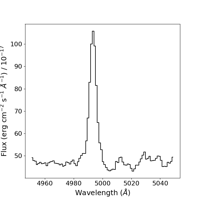
So we now have the data for a region containing only the Hβ line and some continuum noise either side of it. We can begin to create our model for the data. In this case, we'll use a first-order polynomial to fit the continuum around the line, and a Gaussian distribution for the emission line itself - we'll use AstroPy models to do this. Once our models are defined and we've provided initial guesses for the Gaussian parameters, we'll combine them to create a total model for the continuum and emission line:


                # use AstroPy to define our models, and give initial guesses for the Gaussian parameters 

                cont = models.Polynomial1D(1) 

                g1 = models.Gaussian1D(amplitude=110, mean=4990, stddev=10) 

                

                # define the total model to fit to our data: the continuum and emission line 

                g_total = g1 + cont

This gives us a total model, g_total, consisting of a polynomial and a Gaussian distribution with an initial guess at the parameters. Here, amplitude is the amplitude of the emission line, mean is the centroid wavelength of the Gaussian, and stddev is the width (in standard deviations) of the Gaussian.

We need to choose a fitter to use to fit our model to the data: we'll use AstroPy's LevMarLSQFitter - a least squares method - for this. We'll also define an array of wavelength values that has a much higher step number so we can nicely plot our resulting fit over our data.


                # define the fitter

                fit_g = fitting.LevMarLSQFitter()

                # fit the model to the data 

                g = fit_g(g_total, w_hb, flux_hb, maxiter = 1000) 

                

                # define an array of wavelength values across our wavelength range with 
a high number of steps, to plot our model over our data 

                x_g = np.linspace(np.min(w_hb), np.max(w_hb), 10000) 

                

                # plot the model and the data 

                plt.figure(figsize=(7,7)) 

                plt.step(w_hb, flux_hb, where='mid', color='k') # plot the data 

                plt.plot(x_g, g(x_g), color='red') 

                plt.xlabel(r"Wavelength ($\AA$)", fontsize=18) 

                plt.ylabel(r"Flux (erg cm$^{-2}$ s$^{-1}$ $\AA^{-1}$) / 1e-17", fontsize=18) 

                plt.xticks(fontsize=16) 

                plt.yticks(fontsize=16) 

                plt.show()

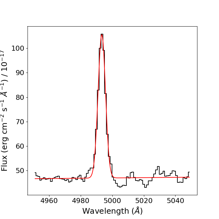
We can call the parameters of the final fit using the .parameters property of the fit g, and calculate uncertainties on these parameters by taking the square root of the diagonal of the covariance matrix.


                # call the parameters of the final fit 

                print(g.parameters) 

                peak, mean, width, m, c = g.parameters 

                

                >[5.85994682e+01 4.99338565e+03 2.34749075e+00 1.60481558e+01
                6.18933598e-03]

                

                # calculate the standard deviation from the final fit values by taking the
 square root along the diagonal of the covariance matrix 

                fit_errs = np.sqrt(np.diag(fit_g.fit_info['param_cov'])) 

                peak_err, mean_err, width_err, m_err, c_err = fit_errs 

                

                >[1.15855157e+00 5.34880217e-02 5.43317087e-02 3.34500609e+01
                6.68883712e-03]

The amplitude and mean of the Gaussian can be used to calculate the area under the Gaussian - since the Gaussian is modelling the Hβ line, then the area under it is a measure of the line flux, often denoted by F(Hβ) for Hβ. The equation for the area underneath a Gaussian profile is the integral of the formula of a Gaussian distribution.

Lets define a function to calculate the line flux using the formula for the area under a Gaussian, and the uncertainty on the line flux using error propagation.


                # create a function for calculating line flux and the associated uncertainty

                def line_flux(peak, width, peak_err, width_err): 

                flux = peak * width * np.sqrt(2*np.pi)

                flux_err = flux*np.sqrt((peak_err/peak)**2 + (width_err/width)**2) 

                return flux, flux_err 

                

                # call the function with the parameters and errors from the Hβ line fit 

                line_flux(peak, width, peak_err, width_err) 

                

                >(344.8160702109391, 10.49596528607543)

That is thus the line flux (and associated uncertainty) of the Hβ line in our spectrum. Lets now repeat the entire process, but this time for the [SII]λλ6717,6731 doublet.


                # use numpy array slicing to select region around [SII] doublet 

                sii_sliced_index = np.where(np.logical_and(w>=6850, w<=6980)) 

                w_sii = w[sii_sliced_index] 

                flux_sii = flux[sii_sliced_index] 

                

                # plot the doublet 

                fig = plt.figure(figsize=(7,7)) 

                plt.step(w_sii, flux_sii, where='mid', color='k') 

                plt.xlabel(r"Wavelength ($\AA$)", fontsize=18) 

                plt.ylabel(r"Flux (erg cm$^{-2}$ s$^{-1}$ $\AA^{-1}$) / $10^{-17}$", fontsize=18) 

                plt.xticks(fontsize=16) 

                plt.yticks(fontsize=16) 

                plt.show()

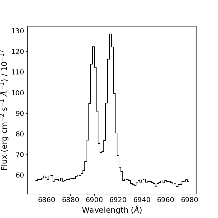
This time, there's a complication: the two lines in the doublet are blended: their line profiles overlap each other considerably. Therefore, to ensure our Gaussian fits are reasonable, we will need to apply some additional constraints to our fitting proceedure.

From atomic physics, we know that the wavelength seperation between the two lines in the doublet is about 14Å, which we will need to correct for the redshift of the object. We also know that, since the two lines are emitted by the same ion (i.e. SII), the lines must have the same line widths, as they must be emitted by the same gas. We can apply these constraints to our fits by tying the properties of the two Gaussians in the total fit using Python functions.


                # create functions to tie the means and widths of the gaussian fits 

                def tie_mean(model): 

                return model.mean_0 + 14*(1+z)

                def tie_width(model):

                return model.stddev_0

Now, lets create our two-Gaussian model, apply our contraints by using the .tied property with the functions we've written, and fit the data and plot the results as before.


                cont = models.Polynomial1D(1) 

                g1 = models.Gaussian1D(amplitude =120, mean=6895, stddev=2) 

                g2 = models.Gaussian1D(amplitude =130, mean=6915, stddev=2) 

                

                g2.mean.tied = tie_mean 

                g2.stddev.tied = tie_width 

                

                g_total = g1 + g2 + cont 

                

                fit_g = fitting.LevMarLSQFitter() 

                g = fit_g(g_total, w_sii, flux_sii, maxiter = 1000) 

                

                x_g = np.linspace(np.min(w_sii), np.max(w_sii), 10000) 

                

                # plot the model and the data

                plt.figure(figsize=(7,7))

                plt.step(w_sii, flux_sii, where='mid', color='k')

                plt.plot(x_g, g(x_g), color='red')

                plt.xlabel(r"Wavelength ($\AA$)", fontsize=18)

                plt.ylabel(r"Flux (erg cm$^{-2}$ s$^{-1}$ $\AA^{-1}$) / $10^{-17}$", fontsize=18)

                plt.xticks(fontsize=16)

                plt.yticks(fontsize=16)

                plt.savefig("sii_fit.png")

                plt.show()

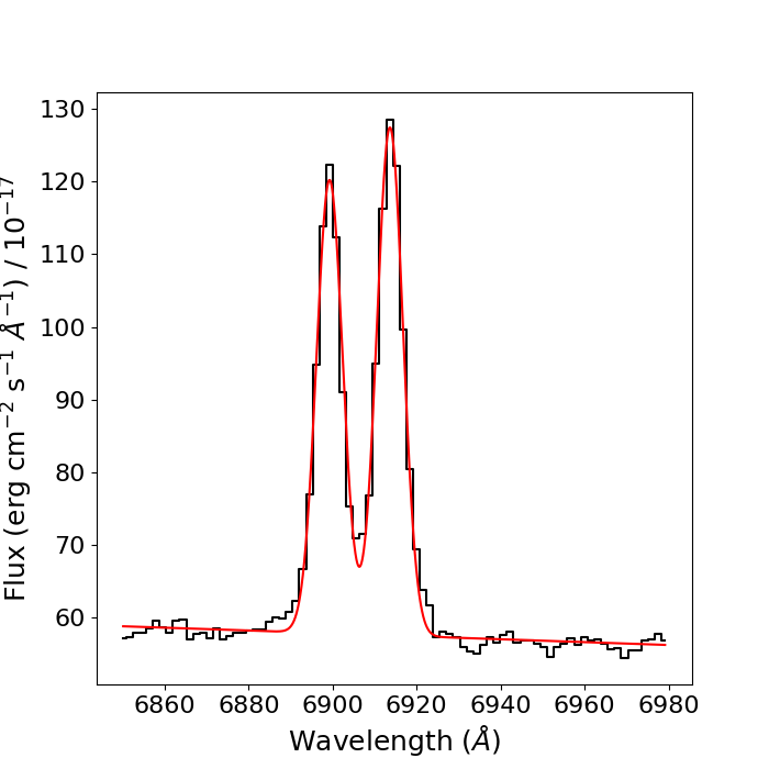
We now have the [SII] doublet fitted! Lets now calculate the line flux for each line in the doublet. A word of warning here: since we have constrained the mean and width of the [SII]λ6731 line to that of the [SII]λ6717 line, the fit does not give uncertainties for the mean and width of the [SII]λ6731 line. However, since these parameters are constrained, these uncertaines are the exact same as they are for the [SII]λ6717 line; we'll use these to calculate the line flux errors, as seen below.


                # call the parameters of the fit 

                print(g.parameters)

                peak_1, mean_1, width_1, peak_2, mean_2, width_2, m, c = g.parameters

                

                # calculate the standard deviation from final fit, but be careful of constraints!

                fit_errs = np.sqrt(np.diag(fit_g.fit_info['param_cov']))

                peak_err_1, mean_err_1, width_err_1, peak_err_2, m_err, c_err = fit_errs

                

                line_flux_sii6717 = line_flux(peak_1, width_1, peak_err_1, width_err_1)

                line_flux_sii6731 = line_flux(peak_2, width_2, peak_err_2, width_err_1)

                

                print("[SII]6717 line flux = ", line_flux_sii6717)

                print("[SII]6731 line flux = ", line_flux_sii6731)

                

                >[SII]6717 line flux =  (488.51102128425913, 9.221833755704399)

                >[SII]6731 line flux =  (547.2816480064968, 9.743237446490088)

So, we now have line fluxes for the Hβ emission line and the [SII]λλ6717,6731 doublet. But what can we actually do with them? Read on...

Example: deriving the electron density of the gas

The reason why astronomers are so interested in measuring line fluxes from a variety of emission lines is that they can be very powerful tools for determining properties of the line-emitting gas. To give a few examples, we can use line fluxes to calculate gas masses, electron densities, temperatures, ionisation states, and ionisation mechanisms. In this section, I will give a brief introduction to the theory behind some of these methods, and show how we can implement them using the PyNeb python module.

Let's begin by using our [SII]λλ6717,6731 line fluxes to determine the electron density of the gas in this galaxy.

Note: for a comprehensive introduction to using emission lines to determine physical properties of astrophysical gas, see `Astrophysics of Gaseous Nebulae and Active Galactic Nuclei' by Osterbrock & Ferland, which is (in my opinion) the master textbook for this kind of work.

Important note: the [SII]λλ6717,6731 density technique has (in my opinion) severe limitations in many cases. Therefore, alternative and more robust methods should be used where possible (see Holden et al. 2023 for details).

Collisions between atoms (or ions) in a gas cloud cause electrons in those atoms/ions to gain energy and jump to a higher energy level in a process called collisional excitation. A higher-density gas will have a higher rate of collisional excitation. After a certain amount of time (set by the radiative transition probability), a collisionally-excited electron will radiatively de-excite, emitting a photon and returning to the lower energy level. However, electrons may also be de-excited by collisions between atoms/ions - this is called collisional de-excitation. If the gas density is high enough, then the timescale for collisional de-excitation will be much shorter than that of radiative de-excitation, and so very few photons will be emitted from downward transitions.

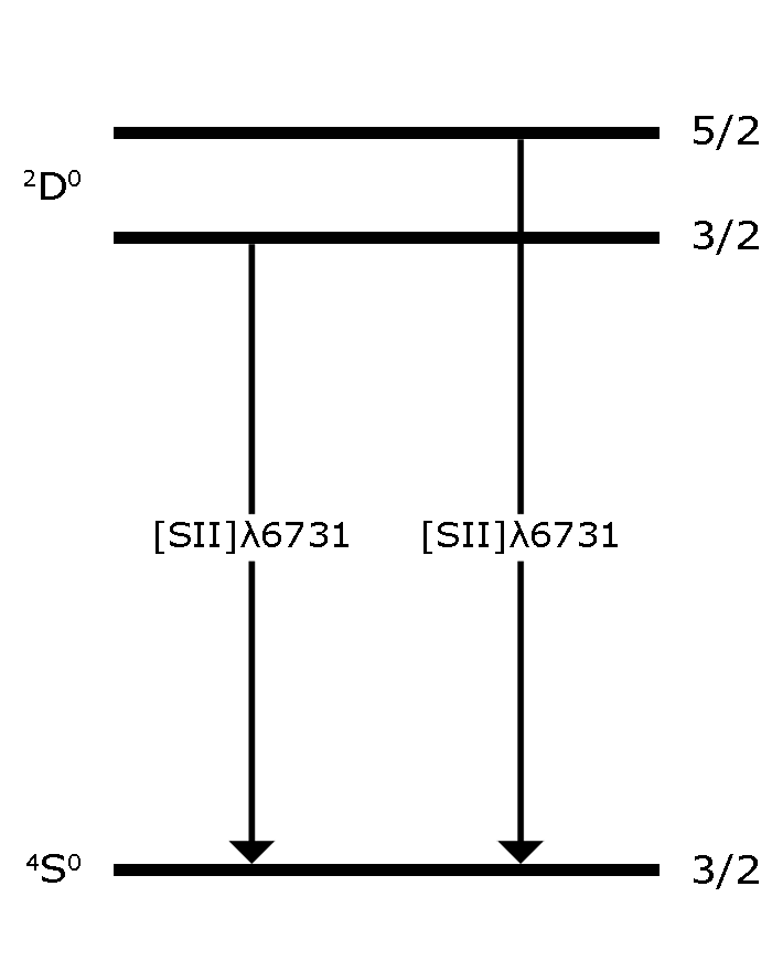
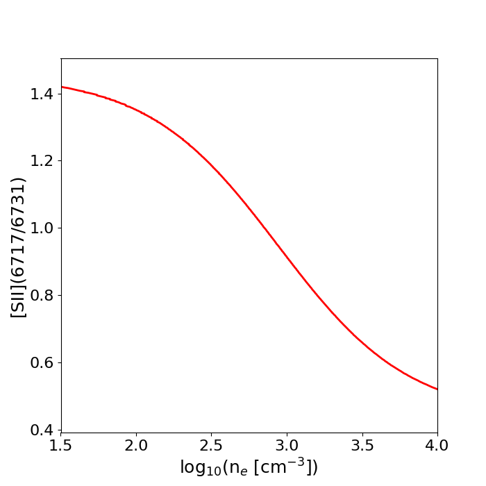
Figure 1: Energy-level diagram for the [SII]λλ6717,6731 doublet. Note that the upper energy levels of the lines are closely-spaced, and that they share the same lower level.

We can define a `critical density' for a given transition within an ion: this is the electron density for which the rates of collisional and radiative de-excitation are approximately equal. The relative strength of two emission lines that arise from transitions from closely-spaced upper energy levels to the same lower energy level will not depend too much on temperature, but will strongly depend on the density of the gas and the critical densities of the transitions. Therefore, by measuring the flux ratio of two such emission lines (such as the [SII]λλ6717,6731 doublet; see Figure 1), we can determine the electron density of the gas by comparing the measured ratio to that expected from atomic physics - this is perhaps made clearer by plotting the variation of the [SII]λλ(6717/6731) ratio against electron density:

Figure 2: Variation of the [SII](6717/6731) ratio with electron density for an electron temperature of T=10,000K. The strong dependence of this ratio on density allows its use as a density diagnostic. This plot was generated with the PyNeb python module.

Calculating the density from the [SII](6717/6731) ratio by hand isn't straightforward, and requires quite a lot of mathematics and atomic physics data. Fortunately, we can use the PyNeb python module to handle all of this for us. However, as an important side-note, I personally believe that it is important to understand how different programs and computational functions work (rather than treating them like magical `blackboxes', in which data goes in and results come out), and so I absolutely recommend learning the underlying physical theory behind this - see Chapter 5 of Osterbrock & Ferland. I also recommend reading the extremely helpful PyNeb manual.

To get started, import PyNeb and create an `Atom` object for the SII ion:


                import pyneb as pn

                

                S2 = pn.Atom('S',2)

To use the Atom class to calculate the electron density, we'll need a few things: the measured [SII](6717/6731) ratio, the temperature of the gas, and the wavelengths of the two [SII] transitions we wish to use. We have already measured the line fluxes for each line in the ratio, so calculating the line ratio is just a case of simple division and error propagation: from our measured fluxes, we find [SII](6717/6731) = 0.89+/-0.02. For the temperature of the gas, we'll assume a temperature of T=10,000K, which is fairly typical for a narrow line region of an active galaxy (although of course, you should always determine the temperature using other line ratios where possible, for example with [OIII](5007+4959)/4363). Finally, we select the two transitions to be those involved in the [SII] ratio we're using. We can now put this all together using the Atom class's `getTemDem' method.


                ne = S2.getTemDen(int_ratio=0.89, tem=10000, wave1=6717, wave2=6731)

		

                print("log_ne = {}".format(np.log10(ne)))

                >log_ne = 3.0407150764688997

As we can see from Figure 2, our [SII] ratio corresponds to an approximate density of ~1000 cm^-3: as expected, our calculated density from PyNeb is close to this.

Closing remarks

Now you should (hopefully) be able to fit Gaussian profiles to emission line spectra and measure line fluxes, as well as have a basic understanding of how to measure electron densities of the emitting gas. It is important to note that this tutorial is only intended to teach how to measure line fluxes, and give a basic understanding of how they may be used to derive the properties of gas. In reality, there are many complications involved - particularly regarding electron densities - which should be taken into account. Namely, be very careful when using the [SII]λλ6717,6731 (and similar) ratios.

Update 22/03/2023: I've made a few small changes (mostly emboldening certain sentences) to highlight that this tutorial is only intended as a basic introduction to line fitting - with examples -, and that deriving actual gas properties requires more care.

Luke Holden